Towards a Probabilistic Disentanglement of Transformer Activations Part 2
This is the second post in our series dedicated to exploring methods around dictionary learning, and the possibility of a probabilistic take on the disentanglement of transformer activations into interpretable monosemantic features.
Building from the first post, we introduce some of the most relevant behaviors around high-dimensional neural-like data and the training dynamics of a sparsity-penalized Autoencoder with an overcomplete basis.
Replication code is based on the GitHub repo GitHub, but with important modifications to ensure consistent replication and logging of the experiments.
Setup of the experiment
In this post, we will keep working with a synthetic dataset of neural-like activations, generated in a similar fashion as the first post in the series.
Taking as a reference the Conjecture initial article, we will use 2 different dataset generation methodologies.
1) Generate the ground truth features with decay in their probability occurrences, this will replicate a property that real activations likely have. This means some features will probably be way more likely than others.
- The feature
is_frenchprobably is way more likely than the feature@_is_python_decorator.
2) Generate the ground truth features with decay and correlation. This tries to extend the behavior of the first data generation method to include another property that real activations probably have. This means that some features co-occur with a higher probability than others.
- For example, the feature
is_frenchprobably co-occurs with the featureword_is_gendered, due to the fact that French have gender-variant nouns.
Parameters of the experiments
| Parameter | Value |
|---|---|
| Activation Dimensionality | 256 |
| Number of ground truth features | 512 |
| Feature probability Decay | 0.99 |
| Average number of features per sample | 5 |
All the experiments will be performed on both data generation methodologies.
Dataset Exploration
To introduce the datasets generated, we created some visualizations to get intuitions on the effect of some of the parameters.
When working with high-dimensional data, it’s important to generate helpful and understandable visualizations.
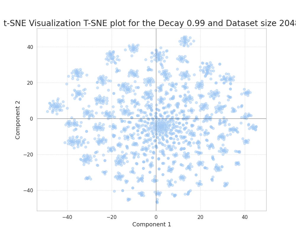
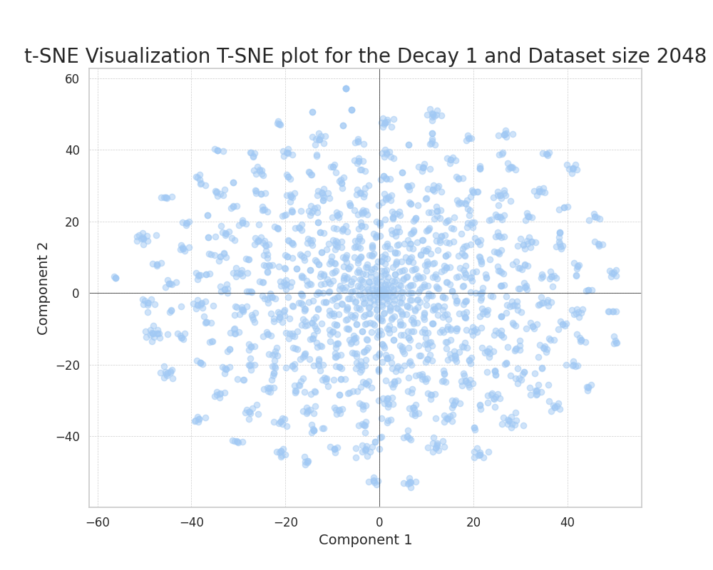
We used t-SNE (t-distributed stochastic neighbor embedding) to project down to two dimensions the 256-dimension dataset.
With this, we mainly wanted to explore the variation of the feature probability decay and the correlation, or lack thereof, between the ground truth features.
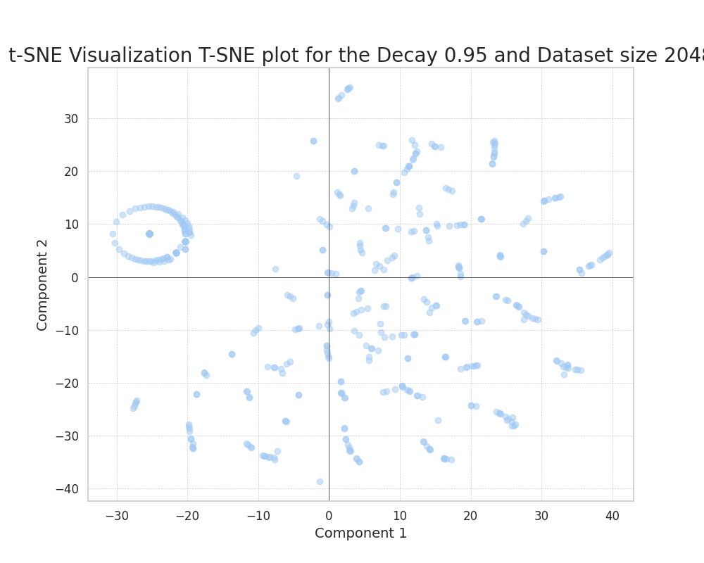
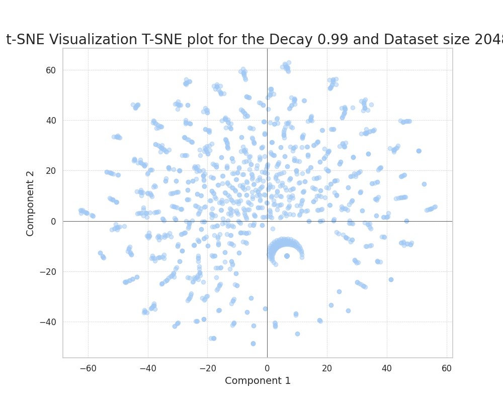
Uncorrelated features
 |
 |
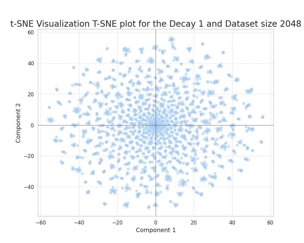 |
We can see how, as we increase the decay, the data points tend to evenly distribute in the plane.
This is because, as the features have equal probabilities, there is no way of embedding their distances in a more compressed way. The small agglomerations of points in the later plot should not be confused with single features. They are superpositions of randomly close features that happen to co-occur.
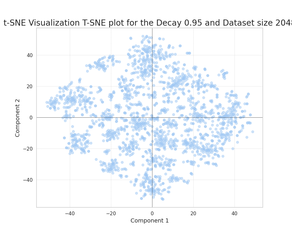
Correlated features
 |
 |
 |
In the case of correlated ground truth components, we can also observe how, as we increase the feature probability decay, the points more evenly distribute in the plane.
An interesting phenomenon can be observed, clearly distinct from the uncorrelated case. This is the formation of clearly defined clusters in the plane.
This can only be attributed to the correlation of ground truth features; this correlation results in the formation of clusters that efficiently embed the presence of predominantly correlated features in a set of datapoints.
We can see how this phenomenon evolves through the increase of the decay. We observe how the clusters become more compact and frequent as we increase the feature decay. This is because the presence of really common features acts as a way of reducing the noise in the encoding process.
Baseline Methods
To assess the performance of the disentanglement process of the SAEs (Sparse Autoencoders), we define and test some widely used methods for disentanglement that have trivial implementations and do not require costly training.
We use the MMCS metric defined in the previous post to assess the performance of these baseline methods.
Performance
| Method | MMCS | Feature Correlation |
|---|---|---|
| KMeans | 0.56 | No |
| KMedoids | 0.21 | No |
| PCA | 0.17 | No |
| ICA | 0.17 | No |
| KMeans | 0.59 | Yes |
| KMedoids | 0.45 | Yes |
| PCA | 0.18 | Yes |
| ICA | 0.19 | Yes |
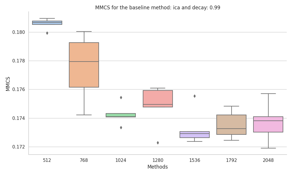
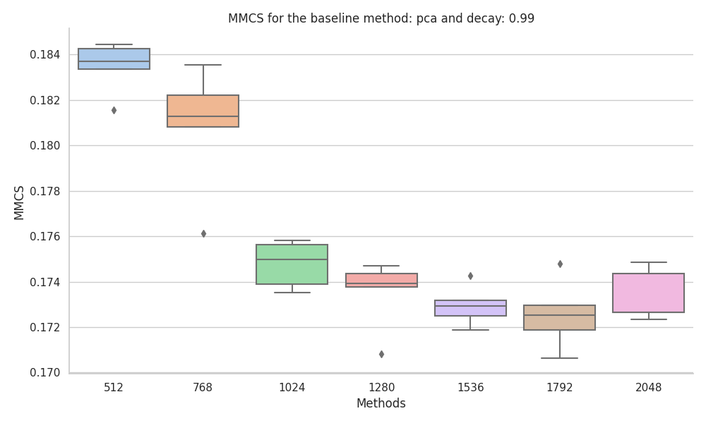
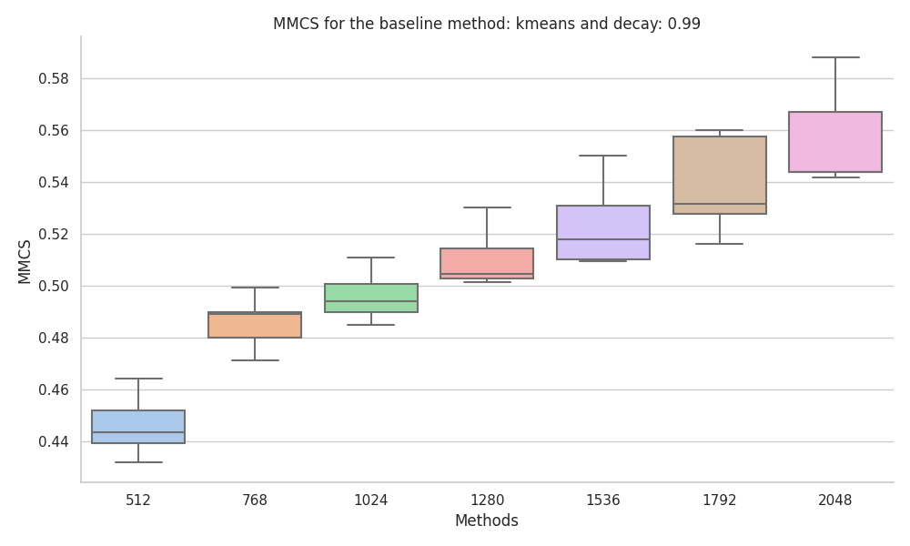
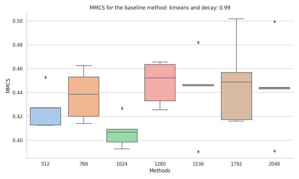
To make sure that the performance was stable relative to the dataset size we ran the baseline methods across a set of dataset sizes.
Uncorrelated features
 |
 |
 |
 |
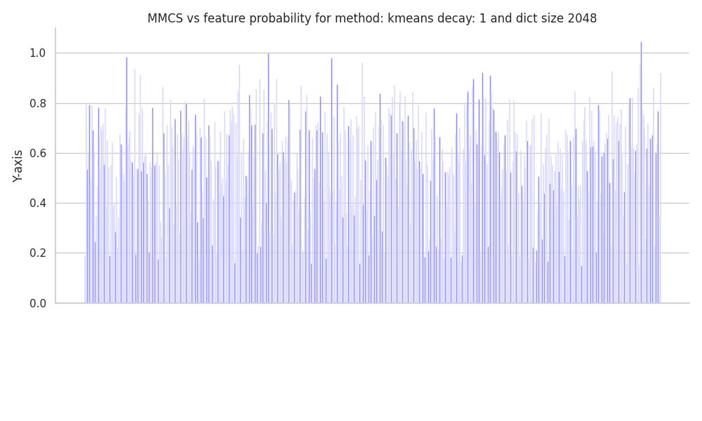
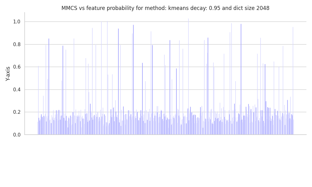
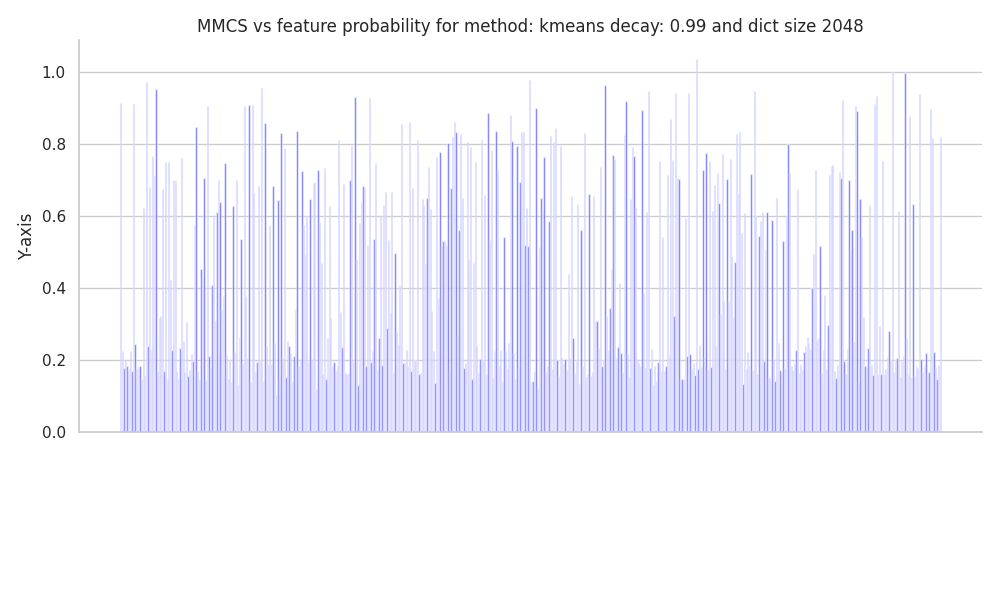
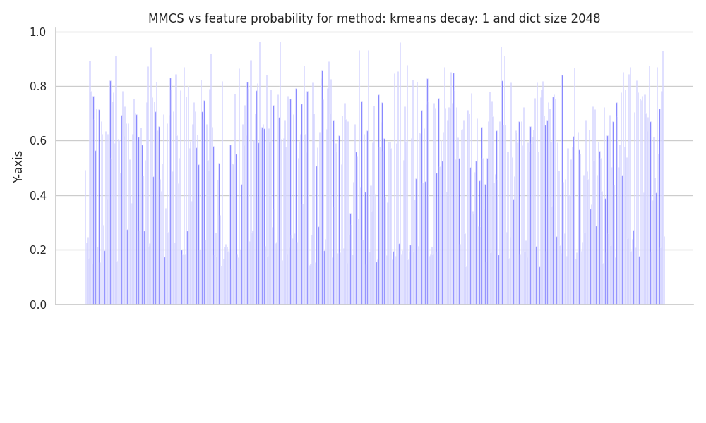
The baseline method that has the best performance on uncorrelated neural-like activations is k-means, with an increase in MMCS with data size, the MMCS converged to around 0.55 when tested up to 409,600 data points.
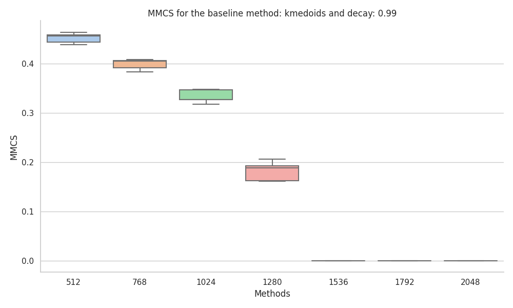
We found the KMedoids implementation in scikit-learn to be very unstable, especially when the ground truth features had different probabilities. Also, during the experiments, we encountered random errors and artifacts.
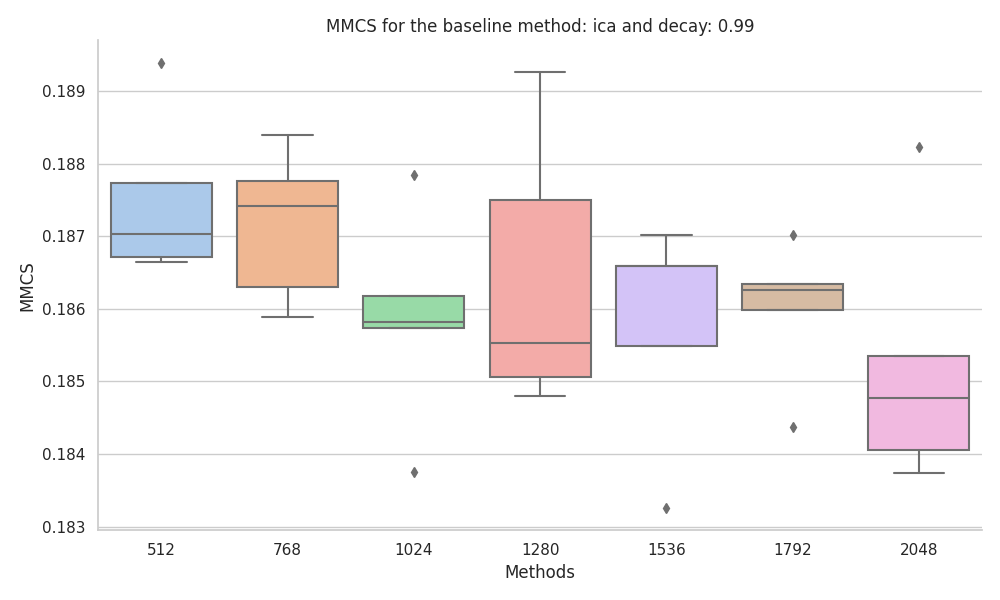
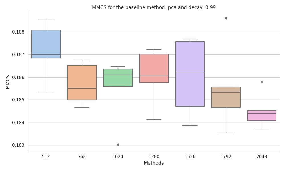
The last two methods, PCA and ICA, were found to not be suitable for the task due to the fact that they just retrieve linear combinations of the most frequent features.
Correlated features
 |
 |
 |
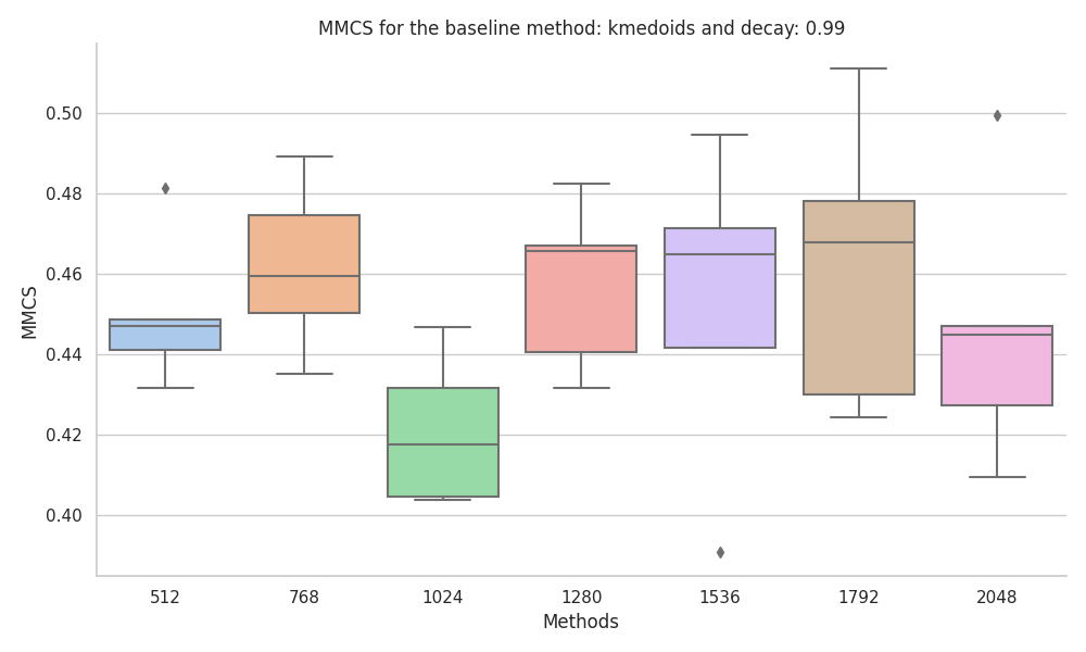 |
When experimenting with the dataset with correlated features, we found that the MMCS where more stable to changes in the dataset size, with KMeans and KMedoids being the best performing baseline methods.
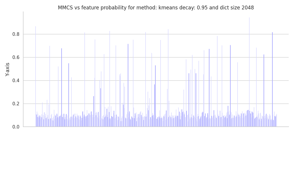
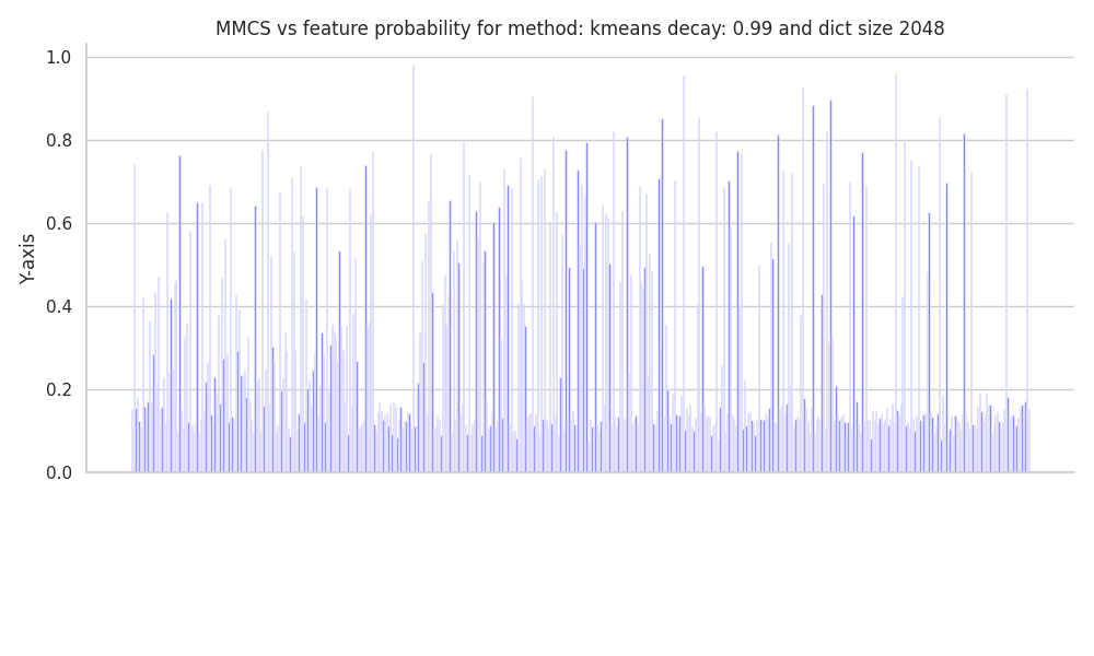
Featuers Representedness
Uncorrelated features
 |
 |
 |
Correlated features
 |
 |
 |
Trainning of SAEs
We trained a set of Sparse Autoencoders for datasets generated using correlated and uncorrelated ground truth features.
The dataset and SAEs have the following specifications:
| Parameter | Value |
|---|---|
| Activation Dimensionality | 256 |
| Number of Ground Truth Features | 512 |
| Feature Probability Decay | 0.99 |
| Average Number of Features per Sample | 5 |
| $L_1$ Penalty | [0.01, 0.02, 0.03, 0.06, 0.1, 0.18] |
| Dictionary Ratios | [0.25, 0.5, 1, 2, 4, 8, 16, 32] |
| Batch Size | 4096 |
| Epochs | 30000 |
Hence, we trained 48 SAEs for the uncorrelated and 48 for the correlated dataset, for a total of 96.
This large training run was made possible due to the services provided by vast.ai. The runs were conducted on an A6000 for 2 hours, and all the metrics were recorded using the wandb API.
During the training of each SAE, some metrics were recorded; some of them proved to be more interesting than others, primarily:
- MMCS of the decoder w.r.t the ground truth features.
- This is useful to observe the evolution of the disentanglement process.
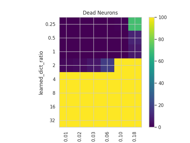
- Number of Dead Neurons:
- This is an important metric presented in the original article. It helps us grasp how efficiently we are using the network’s capacity by recording how many neurons haven’t fired for the last n samples.
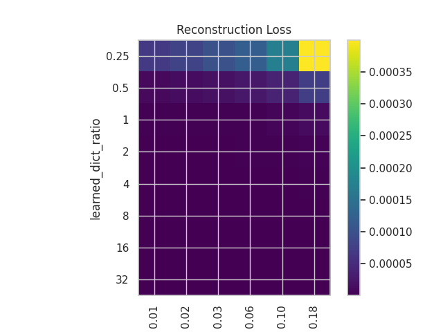
- Recon Loss:
- The reconstruction loss helps us see how well the SAEs are reconstructing the input.
- L1 Loss:
- This helps us assess the sparsity of the activations.
- Metrics for Tracking Feature Learning:
- We set a representativeness threshold to measure the evolution of learned features.
- Learned Features
- Unlearned Features
- Learned Features that have changed dictionary entry
- For all of this, we also kept track of the change in feature representativeness.
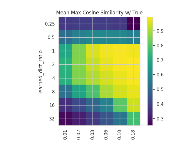
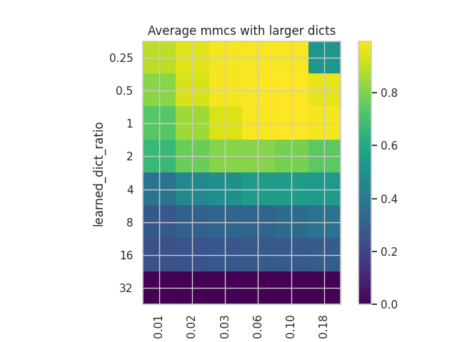
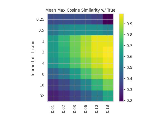
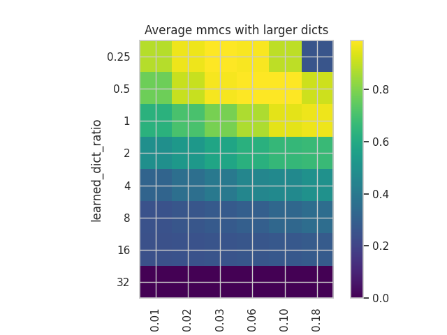
Summary Plots
We plot some of the metrics used in the original paper for both the correlated and uncorrelated datasets. Uncorrelated
 |
 |
 |
 |
Correlated
 |
 |
 |
 |
We can see that while the plots in both cases have similar structures in terms of the distribution of values, the values themselves are somewhat different, with a better reconstruction in the case of the correlated dataset but with a slightly worse MMCS.
These plots show how important the tuning of both hyperparameters is, especially when dealing with correlated and noisy features, as is the case in language models.
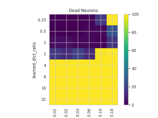
Dead Nuerons
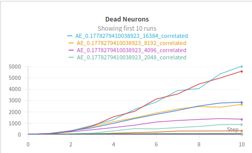
We can observe the phenomenon in whic appropietly sized dictionaries plato the number of dead neurons vs the oversized dictionaries in which the number of dead neurons grow constantly.
This is an important fact that can help us create more efficient SAEs.
Feature tracking plots
We show some of the most intersting figures that show the training dynamics of the SAEs
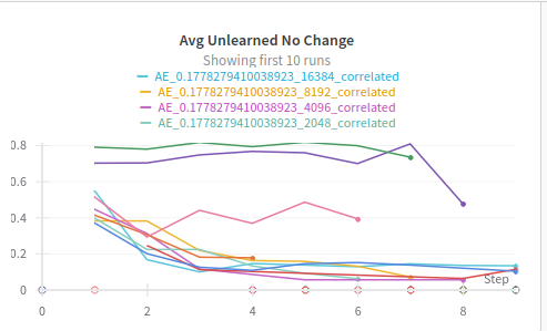
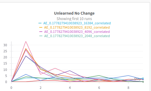
Unlearned Features
One of the most interesting things we observed during training was the phenomenon in which some features where learned to be latter unlearned, we can observe how this was mostly common in undersized dictionaries, probably due to the gradient pressure to learn more important ground truth features .
 |
 |
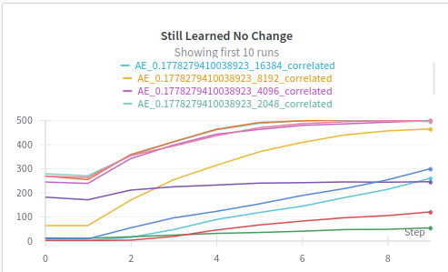
Still Learned Features
Finally we can see how the number of features that are learned and don’t change the entry of the dictionary increases with the epochs, specially for apropietly sized dictionaries with the right $L_1$ penalty.
In the following post, we will explore the possibility of disentangling the features in a probabilistic fashion with the use of Variational Autoencoders, with sparse priors.