Towards a Probabilistic Disentanglement of Transformer Activations Part 1

This is the first of a series of posts where I lay down some intuitions and best practices on how to perform probabilistic dictionary learning on Transformer activations to take features out of superposition.

In the last 6 months, there have been numerous papers and implementations focused on taking the features that compose language models out of superposition.

This first post will be organized in two distinct parts, the first one being the theory and some background information, and the second one in which we will replicate work on Toy Models that will help us in further posts.

Background

In the last decade, enormous advancements have been made in the field of Machine Learning, enabling unheard-of performance in many tasks ranging from computer vision to text generation.

These advancements have sparked interest in how these models perform so well for many reasons such as scientific interest, safety concerns, or capabilities advancement.

Complex models such as Deep Neural Networks have historically been regarded as black boxes, in the sense that it’s not possible to understand the result. This is in contrast to more interpretable models such as decision trees.

The majority of this interest has been focused on Large Language Models, due to the impressive leap in capabilities that they have experienced. Models such as GPT-3 and Llama have shown emerging capabilities such as summarization, coding, in-context learning from just (mostly) unsupervised learning on large corpora of text.

For the aforementioned reasons, a field has emerged which tries to understand the behavior of models from the ground-up mechanisms called Mechanistic Interpretability.

One of the main cruxes of Mechanistic Interpretability (from now on M.I.) is that some components of a Language Model (mainly the neurons on the MLP layer) don’t perform just one task, that is: they are not monosemantic, this makes their interpretation much harder or even impossible.

Motivated by this, there have been many efforts in the field to create methodologies that enable the disentanglement of the functions (also called features) of the components of the model.

When talking about these language models, these features might be very diverse and distributed such as:

• This is a common noun.
• This is the end of this phrase.
• This indicates the beginning of a Latex Formula.

There might be hundreds of thousands or even millions of features that a language model uses while language models only have tens or hundreds of neurons.

This phenomenon is called superposition and can be described as the compression of features in a lower-dimensional space, this is made possible by the relative sparseness of the features in language.

Recently, a major breakthrough has enabled the decomposition into individual features; this has been possible through the use of Dictionary Learning, concretely with the use of Sparse Autoencoders with overcomplete Encoders/Decoders.

Chronology of Dictionary Learning in Interpretability

There are 2 papers that share the honor of starting this field, being very close in time and sharing a lot of commonalities in their methodology.

These two papers are:

• From Anthropic: “Towards Monosemanticity: Decomposing Language Models With Dictionary Learning.”
• From Hoagy Cunningham, et al.: “Sparse Autoencoders Find Highly Interpretable Features in Language Models.”

The two papers follow similar methods but applied to different components of the model.

The first paper uses Sparse Autoencoders to learn a representation of features in the MLP layer in 1L language models. The second paper also uses SAE to learn a representation of features in the MLP but in this case, from the residual stream.

From this point on, many papers and articles have been published; the following is a non-exhaustive list.

Title	Authors	Date	Link
Sparse Autoencoders Find Highly Interpretable Features in Language Models	Hoagy Cunningham, Aidan Ewart, Logan Riggs, Robert Huben, Lee Sharkey	19/09/2023	link
Towards Monosemanticity: Decomposing Language Models With Dictionary Learning	Anthropic	04/10/2023	link
Measuring Feature Sparsity in Language Models	Mingyang Deng, Lucas Tao, Joe Benton	11/10/2023	link
IDENTIFYING INTERPRETABLE VISUAL FEATURES IN ARTIFICIAL AND BIOLOGICAL NEURAL SYSTEMS	David Klindt, Sophia Sanborn, Francisco Acosta, Nina Miolane	18/10/2023	link
Features and Adversaries in MemoryDT	Joseph Bloom, Jay Bailey	20/10/2023	link
Some open-source dictionaries and dictionary learning infrastructure	Sam Marks	02/12/2023	link
Some additional SAE thoughts	Hoagy	13/01/2024	link
Case Studies in Reverse-Engineering Sparse Autoencoder Features by Using MLP Linearization	Jacob Dunefsky, Philippe Chlenski, SenR, Neel Nanda	14/01/2024	link
Addressing Feature Suppression in SAEs	Benjamin Wright, Lee Sharkey	02/02/2024	link
Attention SAEs Scale to GPT-2 Small	Connor Kissane, robertzk, Arthur Conmy, Neel Nanda	03/02/2024	link

Method Description

The Disentanglement methods used in Dictionary Learning mainly work on the following principle.

We have a model that, on inference, produces activations in their components, the MLP for example.

Let $x = \mathbb{R}^{d_{mlp}}$ be an activation of the MLP in a given layer and token position for a prompt.

We expect that the activation $x$ is composed of a sparse set of features.

The task is then to reconstruct the activations with a small set of learned features, that we hope are interpretable.

To do so, we use Sparse Autoencoders. These are Autoencoders that try to reconstruct their input (the model activations), but with an added sparsity penalty to promote the use of as few directions as possible.

Given the fact that language is expected to have many more features than there are neurons in an MLP, we use overcomplete SAE.

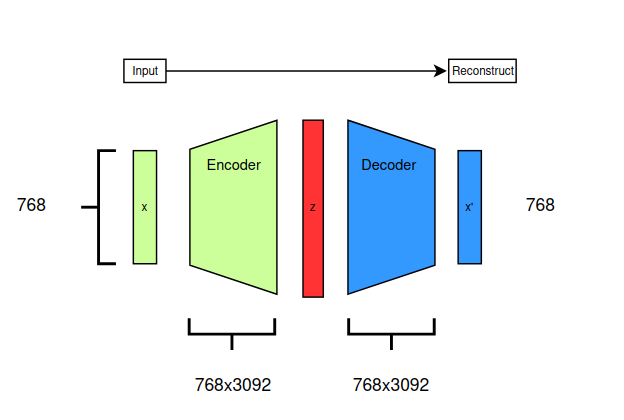
The key trick when learning a Dictionary of features from the activations from a model component’s is to promote sparsity in the activations, this can be done in a number of ways, buy mainly it’s done trough the $L_1$ penalty.

From the original article this translate in the following loss function.

\[\mathcal{L}(x) = \lVert x-\hat{x} \rVert^2_2 + \alpha\lVert c \rVert_1\]

The first term corresponds to the reconstruction loss, and the second term is the $L_1$ penalty controled by the hyperparameter.

Toy Models Replication

This following section will be a replication of the section on Toy Models in link, which will help us establish a baseline for comparison.

Some of the replication code is available on GitHub.

Data Generation

The initial article proposed a data generation process that permitted the controlled generation of Neural-like data, composed of feature vectors with varying probability of presence.

The data generation process is as follows:

1) Generate a set of n ground truth vectors from an m-dimensional sphere. This can be done by the following process: 1) Sampling from an m-dimensional Gaussian, with mean 0 and variance 1. 2) Normalizing the n sampled vectors by dividing them by their norm. 3) This results in a set of n points from the unit sphere. 2) Define the coefficients for each feature in a sample. These coefficients will define the presence or absence of a feature in an activation. To follow the sparsity theme, these coefficients should be 0 with high probability. The process is as follows: 1) Generate a random correlation matrix by sampling from an m-dimensional Gaussian and then making the matrix symmetric and positive definite. 2) We make some features more likely than others by exponentially decaying by feature index. 3) Then we just rescale the feature probabilities to get the desired mean number of features in superposition.

Graphics of the Data Generation

We plot the steps of the feature generation process with n=6 and m=3 to get some intuitions about the task.

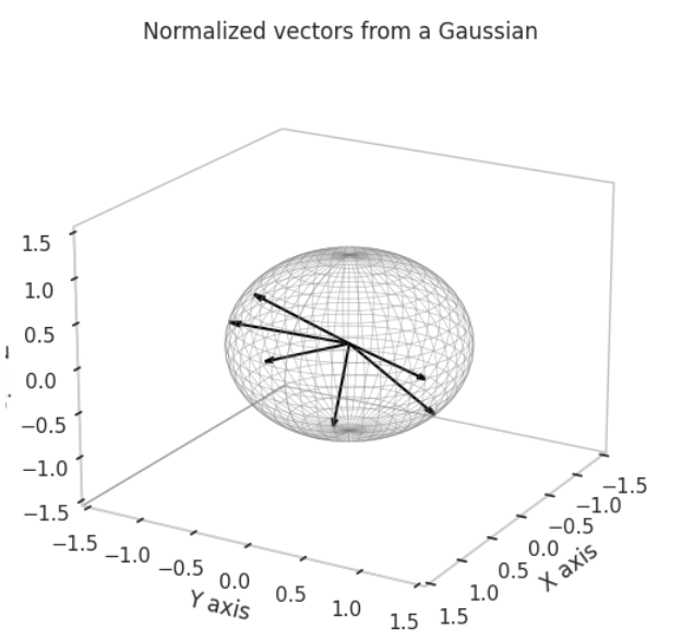
The first step, as outlined above, is to generate a set of ground truth feature vectors, in this case, 6 of dimension 3. In the original toy models, they used 512 of dimension 256. This was chosen to aid with the geometric intuitions.

We sample from a Gaussian distribution with mean 0 and variance 1.

Later we normalize the vectors, so they have norm 1 and the lie in the unit sphere.

Once the ground truth features are constructed, we proceed with the sampling of (Synthetic) Neural Activations that are just a sparse composition of ground truth features, with some perks like a correlation structure to make them behave in a more real way.

As an example, we sample 12 SNAs (Synthetic Neural Activations), and we highlight in green the Ground Truth features that are active in their generation.

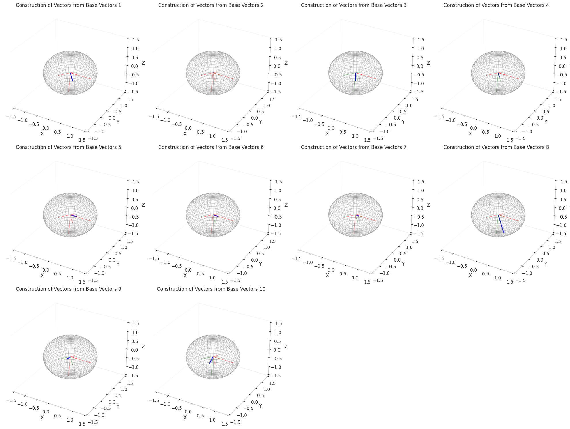
In the plot above, the blue arrows are the sampled activations, the green arrows are the ground truth features that are active, and the red arrows are the inactive ones.

It’s important to note that due to the low dimensionality, some activations have just one Ground Truth Feature being active and hence are superimposed on the Ground Truth Feature.

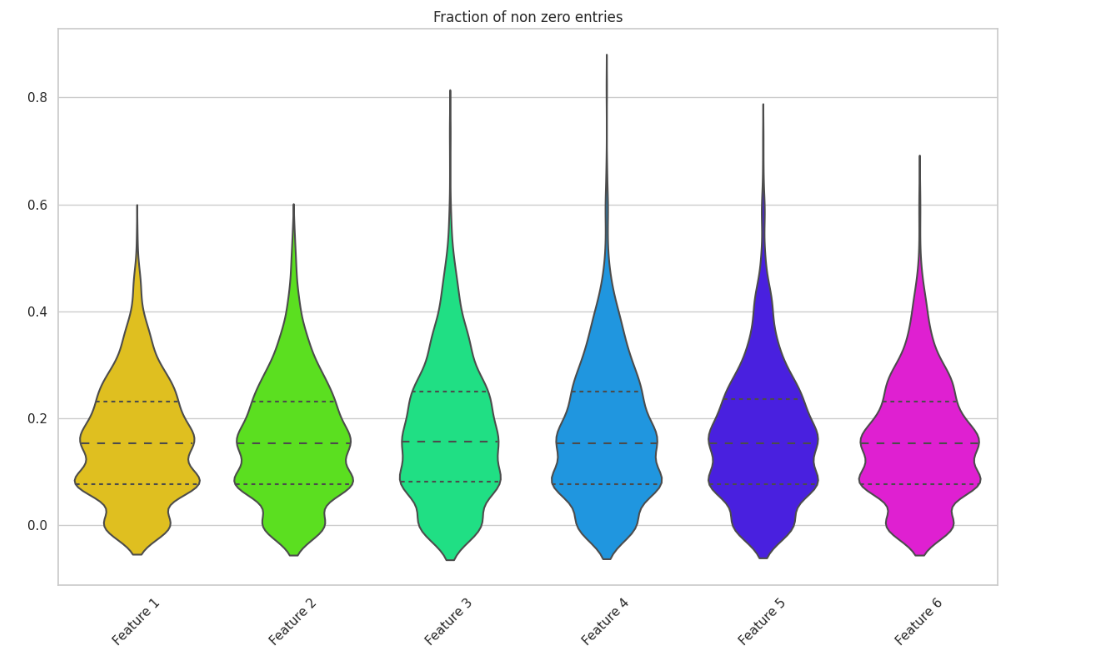
If we plot the frequency of feature activations, we can see that some features are slightly more frequent than others, this is not surprising since we’ve implemented a small amount of decay and we’ve imposed a correlation structure.

These effects are more prevalent when dealing with higher dimensionalities and a greater amount of features.

In training GIFs

We trained a set of 12 Sparse Autoencoders with multiple L1 penalties and Dictionary Sizes

(Note that the dictionary size is nothing more than the Encoder/Decoder size, which for this application is overcomplete, meaning bigger than the input/output.)

We can see some of the outputs, provided by the code in the repo.

From left/right top/down, we can see the plots for:

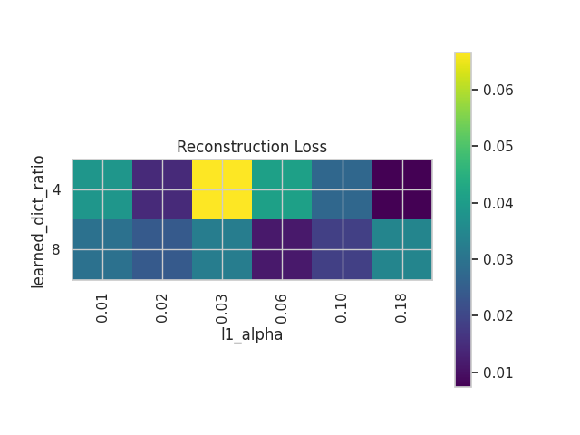
• Reconstruction loss:
  • This is the MSE of the input/output averaged over the whole dataset.
  • We can see how larger dictionary sizes as well as larger L1 penalties produce smaller reconstruction loss.
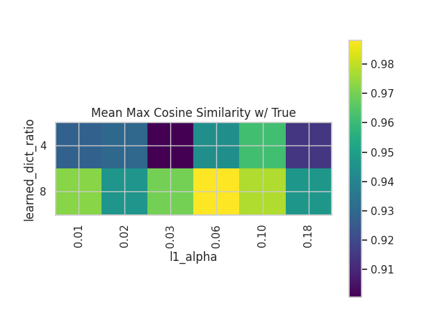
• MMCS:
  • The Mean Max Cosine Similarity is a custom metric widely used in these applications, that helps us understand how well the ground truth features are being recovered.
  • We can see that overall all the SAEs have recovered most of the ground truth features, having a high cosine similarity.
  • For comparison, using PCA the MMCS is 0.42.
• Average MMCS with larger dictionaries:
  • Another way of comparing the performance of an SAE is to compare the recovered features to the ones recovered by larger dictionaries.
  • This is based on the principle that there are many ways of being wrong while there’s only one of being right.
  • Based on the small run for this 3D example, it is difficult to make sense of this plot. We will investigate further in future posts
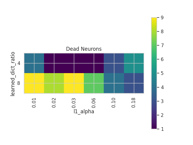
• Number of dead neurons:
  • Dead neurons are a phenomenon in which some neurons in the SAE don’t activate under any input.
  • Keeping track of the number of dead neurons is important for an efficient training of SAEs.
  • We can observe that for the present task there’s a sweet spot in terms of L1 penalty.
  • In regards to the dictionary size, a run with more dimensions and Ground Truth Features would be needed to comprehend the extent to which SAEs are able to retrieve features in superposition.

We can see a visualization of the features being recovered for every SAE run every 10 epochs. We can observe that the majority of the way up to the Ground Truth Features is recovered in the initial iterations. This is mainly due to the simplicity of this toy example with just 3 dimensions and 6 Ground Truth Features.

In the following post, we will explore the dynamics of training for high-dimensionality toy examples, introducing novel techniques like ghost gradients introduced by Anthropic.